Manual¶

Overview¶

The basic procedure of performing a parameter fit with bayesim is as follows:

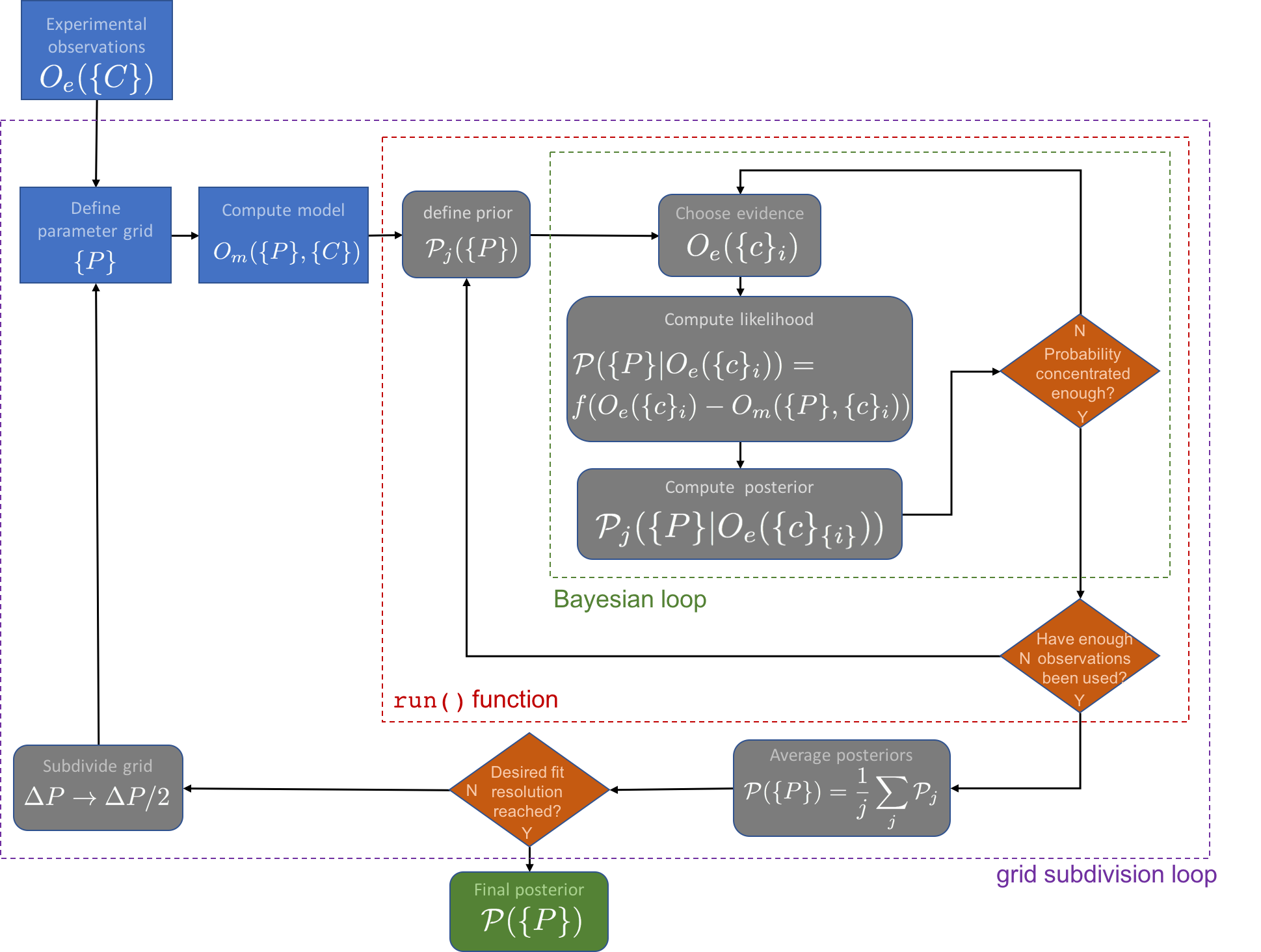
On this page, we will dive into each part of this flowchart in detail to understand what is happening and what options exist to tweak bayesim’s behavior. The code snippets will be assuming that we are modeling a solar cell’s output current \(J\) with two experimental conditions: voltage \(V\) and temperature \(T\).

The first step is to initialize a Model object. Several of the next steps can be rolled into this initialization using keywords, but the only required input is the name of the output variable. For example:

import bayesim.model as bym
m = bym.Model(output_var='J')

Attaching Observations¶

The experimental observations should reside in an HDF5 file with columns for each experimental condition and the output variable. Optionally, there may also be a column for experimental uncertainty. In addition, one should specify one of the experimental conditions (EC’s) to be plotted on the x-axis when visualizing data later on using the ec_x_var keyword. The data are attached using:

m.attach_observations(obs_data_path='obs_data.h5', ec_x_var='V')

If this column isn’t present, the fixed_unc keyword must be passed with a value to use as experimental uncertainty for every data point:

m.attach_observations(obs_data_path='obs_data.h5', ec_x_var='V', fixed_unc=0.02)

By default, to save computational time, bayesim will not import all data points, but rather attempt to maintain some minimum spacing between points such that each piece of evidence is more likely to contribute to constraining the posterior distribution. This behavior can be turned off by passing keep_all=True to the attach_observations() function, and can be tuned using the max_ec_x_step and thresh_dif_frac keywords. thresh_dif_frac is given as a fraction of the range of values of the output variable and defaults to 0.01. It defines the minimum difference in output variable along the x-axis EC (at fixed values of the other EC’s) for which to save a point. max_ec_x_step is the largest step to take in the previously defined x-axis EC before saving a point anyway even if it doesn’t differ by that threshold amount, and defaults to 5% of the range of values of the x-axis EC. Let’s look at an example case where we use the default values for these parameters:

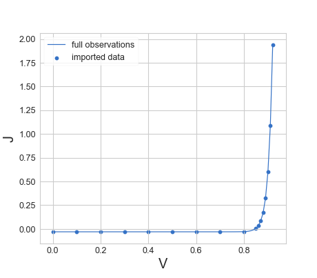
Note how in the ‘flatter’ region of the curve, the spacing along the x-axis of imported points is wider than in the ‘steeper’ region.

Defining Parameters¶

It is possible to predefine the parameter grid by directly constructing a Param_list object and passing it to the Model constructor, although this is not necessary, because bayesim is capable of determining these directly from the model data file (see next step). However, if one wants to use bayesim to generate the list of model points that need to be simulated, this approach is useful. Consider the ideal diode example, where the parameters to be fit were \(B'\) and \(n\):

import bayesim.model as bym
import bayesim.params as byp
pl = byp.Param_list()
pl.add_fit_param(name='Bp', display_name="B'", val_range=[10,1000], spacing='log', length=20, units='arb.')
pl.add_fit_param(name='n', val_range=[1,2], length=20, min_width=0.01)
m = bym.Model(params=pl, output_var='J')

The code block above sets the ranges of values, spacing (linear by default, logarithmic as an option), and number of divisions (10 by default) for the two parameters, and initializes the model object using this parameter grid. We can also set a display name for plot labeling (TeX input is accepted in this field), units (also used in plotting, defaults to ‘unitless’), and minimum width beyond which a grid box won’t be subdivided along this dimension (defaults to 1% of the value range in the appropriate spacing). Some of these parameters can also be set after data import using the set_param_info() function, as in:

m.set_param_info('J', units='mA/cm$^2$')
m.set_param_info('T', display_name='temperature', units='K')

Attaching Modeled Data¶

Next, we need to attach the modeled data. If you’re using bayesim to tell your model what points to run, you can call list_model_pts_to_run() to write out an HDF5 file to pass to your forward model:

m.list_model_pts_to_run(fpath='model_inputs.h5')

You can also directly interface with your model by passing a Python callable, as in:

m.attach_model(mode='function', model_data_func=model_func)

where model_func is a callable in your namespace that accepts dictionaries of inputs, one with keys of the EC’s and one of the fitting parameters (see ideal diode example).

However, typically, the model data will be precomputed and residing in an HDF5 file which will be attached to the model object:

m.attach_model(mode='file', model_data_path='model_data.h5')

The model uncertainty also needs to be computed. This can be done either with a separate function call to calc_model_unc(), or in a single step when attaching the model data:

m.attach_model(mode='file', model_data_path='model_data.h5', calc_model_unc=True)

The model uncertainty calculation can be somewhat expensive for large grids and will be parallelized by default on Unix-based systems.

Performing the Inference¶

Once experimental and model data and their associated uncertainties have been defined and the fitting parameters either explicitly specified or determined from the data, we can do Bayesian inference! The inference is performed by the run() function. Details about what calculations are actually done and what they mean can be found on the Technical Background page; here we will focus on the mechanics of the code.

First, a bounded uniform prior (equal probability in every grid box) is defined. Next, a piece of evidence (one experimental measurement, i.e. in this example a \((V, T, J)\) tuple) is chosen at random. The likelihood at each point in parameter space is computed conditioned on this piece of evidence as a Gaussian in the difference between the measured output and the simulated output at that point, with a standard deviation equal to the sum of the experimental error for that observation and the model uncertainty at that point:

In the ideal diode example, this means more specifically that

This likelihood is multiplied with the prior and normalized to compute the posterior.

Next, bayesim will check if the posterior distribution is “concentrated” enough. This concentration is defined by two optional parameters passed to run(), th_pm and th_pv, both on the interval (0,1) and defaulting to 0.9 and 0.05, respectively. The posterior is sufficiently concentrated is th_pm of the probability mass resides in th_pv of the parameter space. (Entropy-based thresholding is planned as an option for a future release)

If the posterior is not sufficiently concentrated, the posterior is set to the prior, another piece of evidence chosen, and another Bayesian update performed until it is. Once the concentration threshold is met, the posterior is saved and another check is done for whether enough pieces of evidence have been used. The requisite number to use is defined by the min_num_pts keyword in the run() function and defaults to 80% of the total number of observation data points imported. If not enough points have been used, the current posterior is saved, a new uniform prior is set and the process above repeated as many times as necessary for sufficient points to be used. The final posterior is then the average of all computed posteriors. bayesim will inform you how many posteriors were averaged and how many observed data points were used.

Visualizing the Output¶

bayesim has a variety of capacities for data visualization.

Subdividing the Grid¶

Once you have taken a look at your posterior PMF and compared observed and highest-probability modeled data, you’ll have a sense for whether you’d like to go to a higher fit precision by subdividing the parameter space grid. This can be done via a call to the subdivide() function, which accepts one optional argument of threshold_prob, the minimum probability for a box to have in order to be subdivided. It defaults to 0.001. bayesim will then divide every grid box meeting this threshold as well as every box immediately neighboring it into two along every parameter dimension, unless it is already narrower than the minimum width defined for that parameter.

bayesim will inform you how many boxes were subdivided and also automatically save a file of the new points that need to be simulated using the model in order to perform another inference run. This new model data can be attached exactly as described above using the attach_observations() function, and then inference can proceed again.

Miscellaneous¶

m.save_state(filename='statefile.h5')
m = bym.Model(load_state=True, state_file='statefile.h5')