Why bayesim?¶

Probability distributions are nice¶

The output of a bayesim analysis is not just a set of values and uncertainties, but rather a full multidimensional probability distribution. The power of this comes when the regions of parameter space that have highest probability are not simple ellipsoidal blobs with axes along the parameter axes, but instead take on more complicated shapes that can reflect underlying tradeoffs between fitting parameters. For example, in our research group’s first published paper using Bayesian parameter estimation (which used a much earlier precursor of the code that was eventually developed into bayesim), we found that of the four parameters we fit, two were constrained quite well, while two others didn’t seem to be on an individual basis:

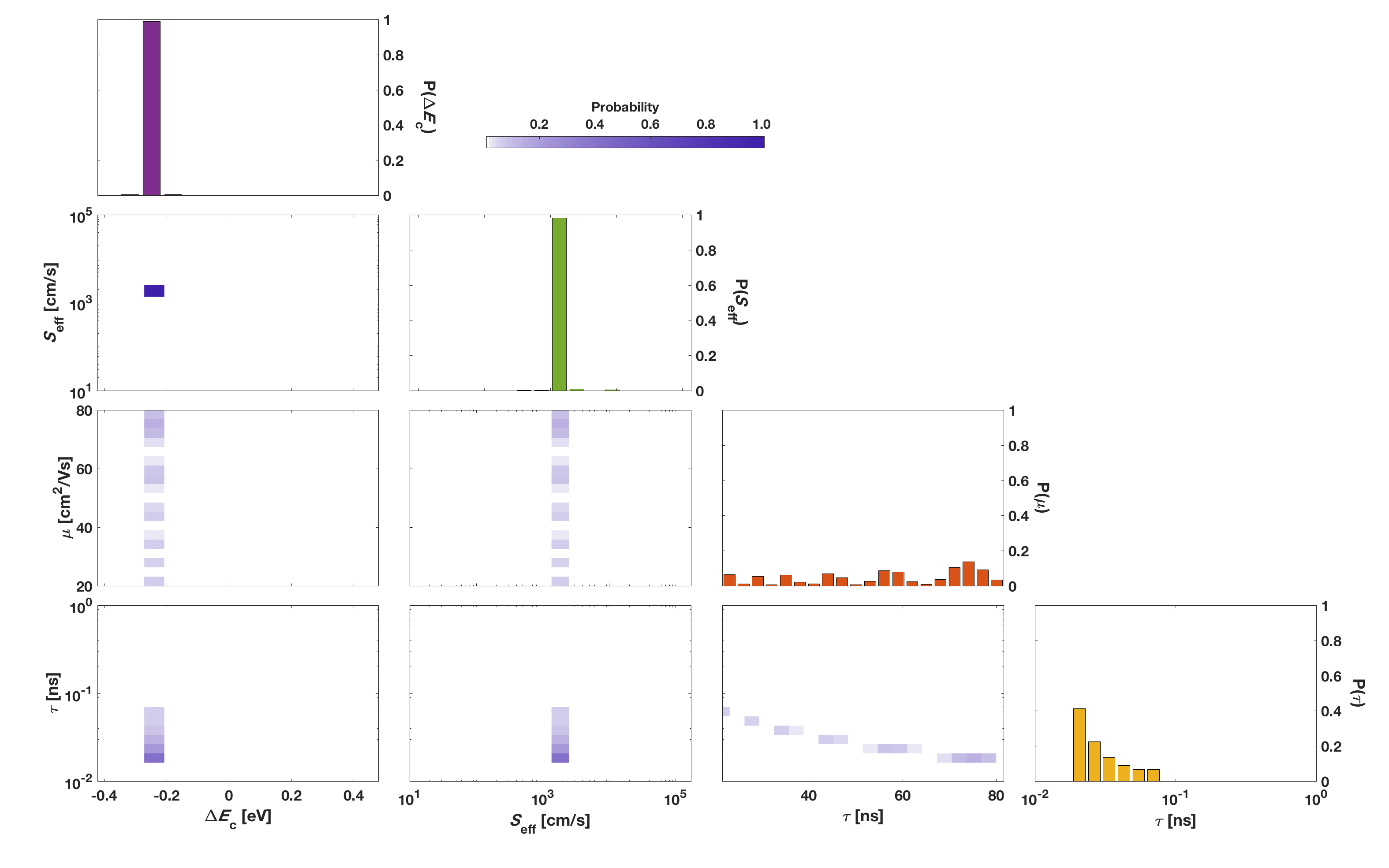
Figure 3 from this paper. The \(\Delta E_c\) and \(S_\text{eff}\) parameters are constrained well, while \(\mu\) and \(\tau\) exhibit a much larger spread in their individual distributions (red and yellow histograms).

However, when we look at the two-parameter marginalization of the final posterior distribution (second plot from the right on the bottom row), we see that while the values of \(\mu\) and \(\tau\) may not have been individually well-constrained, their product was pinned quite well. As it happens, this product is related to a quantity known as the electron diffusion length, and under the conditions we measured the solar cell, other effects that \(\mu\) and \(\tau\) have on performance were small enough that they couldn’t be decoupled from each other.

This type of insight could not be gleaned from a more traditional parameter fitting approach such as a least-squares regression and requires the ability to see the probability distribution over parameters.

Simulations are expensive¶

A very common approach to multidimensional Bayesian parameter estimation involves Monte Carlo (MC) sampling rather than sampling on a grid as we do here. In general, such approaches scale very well to larger numbers of dimensions and hence may have great appeal (“larger numbers” is problem dependent but for “typical” problems if you have more than 10 parameters to estimate, an MC approach is preferable). Bayesim uses adaptive grid sampling, which has two major benefits over MC sampling for relatively low-dimensional problems:

1. It can be significantly less computationally expensive (from a more formal numerical perspective, it avoids the generally large prefactor in cost estimates for MC sampling, which can overwhelm the dimensional savings when the dimensionality is small) and
2. There is significantly less uncertainty that all regions of non-negligible probability are quickly detected, since the coarsest iteration tends to identify all “hotspots” immediately, provided the model uncertainty associated with the sampling density is incorporated.

The take-home message here is that bayesim’s approach shines in situations where the computational effort required to evaluate the likelihood is large, as when the data models are sophisticated numerical solvers, and the number of fitting parameters is (relatively) small.

Many of the Examples we show here involve analytical models, however. This is done only to create examples that are tractable to run in a few seconds on a typical personal computer. In reality, while bayesim certainly works with these models, it is unlikely to be the most efficient approach to fitting their parameters. In addition, with an analytical model, tradeoffs such as the one between \(\mu\) and \(\tau\) described above are generally already apparent from the mathematical form of the model and hence the final probability distribution isn’t necessarily required for such insights.